ZScope

An integrated platform for electrochemical impedance analysis, from measured spectra to physical quantities

Overview · Capabilities · Workflow · Verification · Download · Citation

---

Overview

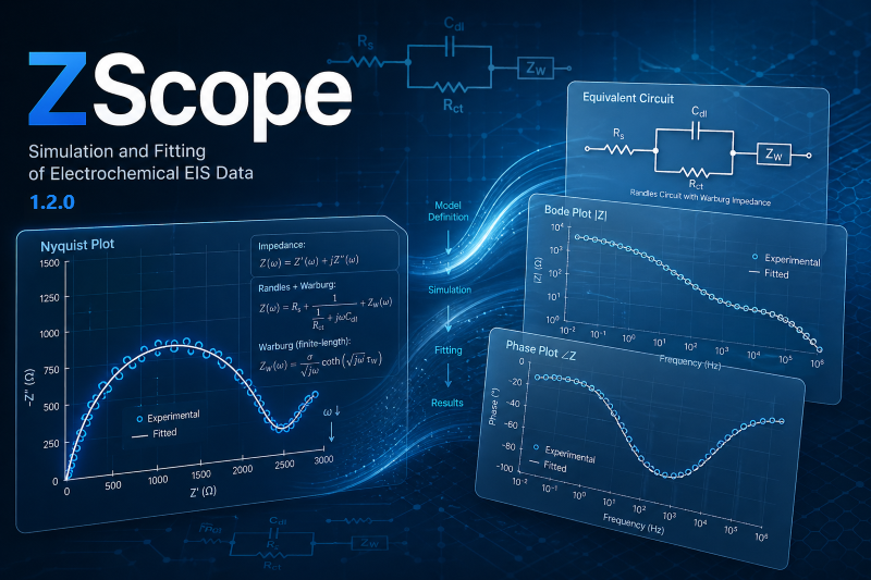
ZScope is a Windows desktop application for electrochemical impedance spectroscopy (EIS) modelling and analysis. It brings circuit construction, interactive simulation, parameter fitting, data validation, uncertainty estimation, distribution-of-relaxation-times (DRT) analysis, and conversion of fitted parameters into physical quantities into one workflow.

The central idea is to keep the circuit, measured spectrum, simulated response, fitted parameters, and reported quantities connected. Build or edit a circuit visually, see how it changes the spectrum, fit it to experimental data, assess the fit and parameter uncertainty, and report derived quantities with their units and assumptions.

ZScope is designed for researchers working with electrochemical systems, materials, devices, and processes. It can be used for applications including solid-state electrolytes and ceramics, batteries, fuel cells, corrosion, coatings, electrochromic materials, and porous electrodes.

Distribution: ZScope is provided as a ready-to-install Windows application. Python does not need to be installed. The application is intended to run locally; this repository is the software's download and documentation page, not a public source-code distribution.

What ZScope can do

Interactive circuit modelling and simulation

• Construct equivalent circuits on a graphical canvas or use circuit notation.
• Simulate the circuit response and update Nyquist, Bode, and phase plots as circuit topology or parameter values change.
• Overlay simulated responses with measured spectra to explore how individual elements influence the result.
• Work with general nodal circuit networks rather than being restricted to simple nested series/parallel expressions.
• Use built-in elements including resistors, capacitors, inductors, constant-phase elements, diffusion elements, Gerischer elements, and transmission-line models.
• Define custom impedance or admittance elements through the interface.

Fitting and model assessment

• Fit circuit parameters to measured complex-impedance data.
• Configure fitting options, parameter bounds, weighting, loss functions, and search strategies.
• Use multi-start and optional global-search approaches to reduce dependence on a single initial guess.
• Compare retained candidate circuits using information criteria such as AICc, AIC, and BIC, where available.
• Inspect residuals and parameter uncertainty rather than relying on a fit curve alone.
• Use optional Bayesian Markov chain Monte Carlo (MCMC) analysis to examine parameter distributions, correlations, and credible intervals.

Data validation and DRT

• Perform Kramers–Kronig (KK) consistency checks to help assess whether a spectrum is compatible with the assumptions used in impedance analysis.
• Calculate a distribution of relaxation times (DRT) using non-negative regularisation.
• Inspect DRT features and use the result to support circuit interpretation.
• Treat validation, fitting, and DRT as complementary analyses: none by itself proves that a chosen circuit is physically unique.

From fitted parameters to physical quantities

• Apply sample-geometry corrections and unit-aware transformations to relevant fitted quantities.
• Calculate quantities such as area-specific resistance, resistivity, and conductivity when the required inputs and assumptions are available.
• Estimate effective capacitance from a constant-phase element using documented conversion approaches.
• Carry units and relevant conventions into the reported results so derived values are easier to interpret and reproduce.

Import, projects, and reporting

• Import measured spectra from supported data files and map frequency, real-impedance, and imaginary-impedance columns.
• Inspect the data and compare measured and fitted responses in the main plots.
• Save a project containing the data and analysis state, then reopen it to continue working.
• Export plots and analysis results for further examination, reporting, and publication preparation.

Workflow

A typical analysis can follow these steps:

1. Import the measured impedance spectrum.
2. Check data consistency using KK analysis and inspect the residual pattern.
3. Construct a circuit using the graphical canvas, circuit notation, or a suitable starting model.
4. Simulate interactively to understand how the proposed circuit responds.
5. Fit the circuit and inspect parameter estimates, bounds, and residuals.
6. Assess uncertainty and model alternatives using the available uncertainty analysis and information criteria.
7. Use DRT as a complementary view of the relaxation behaviour where appropriate.
8. Calculate physical quantities using the relevant geometry, units, and stated model assumptions.
9. Save and export the project, plots, and results.

The steps are a guide rather than a guarantee that every dataset supports every analysis. The appropriate model and the reliability of derived quantities depend on data quality, identifiability, experimental conditions, and physical assumptions.

Verification and limitations

ZScope's numerical methods were tested against synthetic spectra with known parameters and reference calculations. The published software study includes tests of forward circuit solutions, parameter recovery, uncertainty estimates, KK validation, DRT behaviour, and geometry-related transformations.

Examples of verification reported in the study include:

• Circuit solution: a 400-frequency, 11-decade comparison for a delta–star network gave a maximum deviation of approximately (6.2 \times 10^{-15}) between the tested implementations.
• Parameter recovery: 300 synthetic fits across five reference circuits, three noise conditions, and two starting modes converged in the reported test set. Recovery depended on the circuit and noise condition; difficult CPE parameters were less reliably identified.
• Uncertainty estimates: repeated-trial tests compared conventional and robust covariance estimates, including data contaminated with outliers. The robust sandwich estimator improved nominal confidence-interval coverage in the contaminated-data tests.
• KK checks: large-scale synthetic testing examined how detection depends on the size of a distortion relative to measurement noise.
• DRT: tests evaluated peak merging and separation, showing that nearby processes can be unresolved and that peak count and peak parameters should not be interpreted without regard to resolution limits.
• Geometry transformations: numerical tests checked the consistency of unit- and geometry-dependent conversions.

These tests support the implementation of the methods under the tested conditions; they do not establish that every fitted circuit is unique or that fitted elements automatically correspond to distinct physical mechanisms. Correlated parameters, overlapping relaxation processes, noise, model choice, and experimental non-stationarity can limit interpretation. See the paper and Supporting Information for the test designs, quantitative results, and limitations.

Download and installation

Download the latest Windows release

1. Open the latest release page.
2. Download the installer or packaged application provided under Assets.
3. Run it and follow the installation instructions.
4. Start ZScope from the installed application.

A separate Python installation is not required. For release history and older versions, visit the all releases page.

About the download counter

The badge at the top reports the combined download count of assets attached to GitHub Releases across all versions of ZScope. It is provided by GitHub's release-download statistics through Shields.io. It does not count repository clones, page views, downloads from mirrors, or files distributed outside those release assets.

Paper and citation

If ZScope is useful in your research, please cite the software and its accompanying paper. The DOI below is the software archive DOI and is intended to remain stable across releases.

Software DOI: 10.5281/zenodo.20357547

@software{zscope2026,
  author  = {Mohammadi, Tecush and Sharifi, Tayebeh},
  title   = {ZScope},
  year    = {2026},
  version = {3.0.2},
  doi     = {10.5281/zenodo.20357547},
  url     = {https://github.com/Tecush/ZScope}
}

For the exact bibliographic details of the software paper, please use the published article record.

Support and contact

• Issues and feature requests: GitHub Issues
• Developer: Tecush Mohammadi
• Email: tecush@gmail.com
• GitHub: @Tecush

Please include the ZScope version, a short description of the problem, and (where possible) a minimal example or project file when reporting a software issue. Remove confidential or sensitive experimental information before sharing files.

---

Built for researchers who want to connect impedance models with interpretable results.